VLOOKUP

In this post, we are going to discuss about VLOOKUP in Microsoft Excel. The “V” in VLOOKUP stands for vertical. It is a very important function which can be used for finding data from sets of data which are in one or more columns.

Syntax for VLOOKUP:

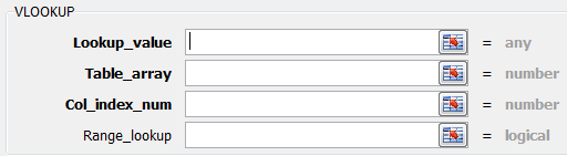
lookup _value: The value we want to find in the first column of the table_array.

table_array: This is the table of data that VLOOKUP searches to find the information we are looking for.

col_index_num: The column number in the table_array that contains the data we want returned.

range_lookup: A logical value (TRUE or FALSE only) that indicates whether we want VLOOKUP to find an exact or an approximate match to the lookup_value. Typing False will return exact matches only.

Let’s see how it actually works.

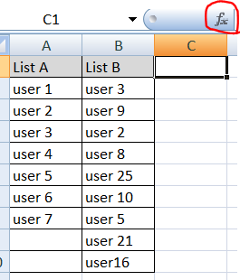
• Suppose, we have two lists of users (say list A and list B) and we want to know what all users in list A are present in list B also.

Below are the two lists in excel:

Let’s do a VLOOKUP to find this. We can either directly write the formula for VLOOKUP (as shown below) or we can use the function field (fx) to insert the function for vlookup using vlookup window:

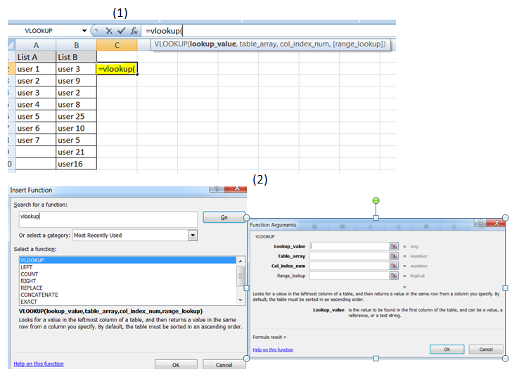
Let’s do the vlookup for finding those values which are in List A in the List B. We will try it using the vlookup function argument (Option 2 above).

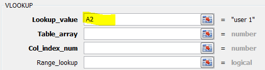
Click on cell C2 and execute function vlookup to get the vlookup window. The first value in List A is user 1 which is in cell A2. Since this needs to be searched first, we will insert A2 in lookup_value.

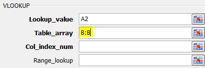
Now place the cursor on Table_array text box in vlookup window.

Since value user 1 can be present in any of the cells in List B, we need to select the whole column B. As soon as column B is selected, the value in the text box Table_array automatically gets updated with B:B.

Now place the cursor in the text box for Col_index_num. Since column B is the only column where we are trying to find data, insert 1 in this text box.

Finally insert value False in Range_lookup text box (since we are searching for the exact value)

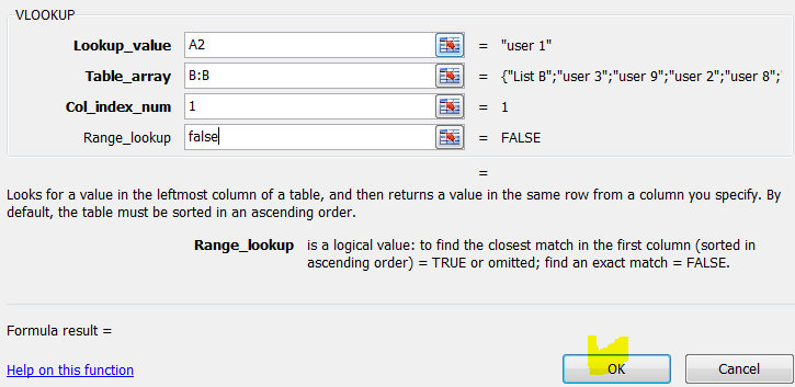Click OK.

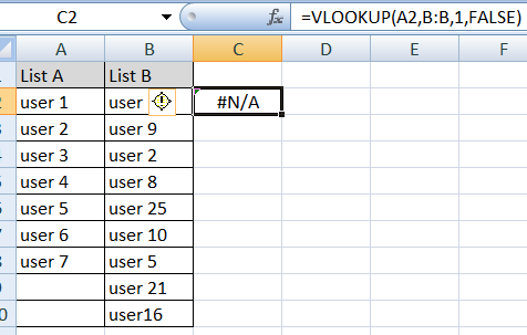We got #N/A in cell C2 which suggests that value user 1 is not present in List B. Now click on bottom right corner of cell C2 to get the following:

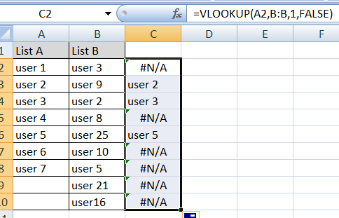This screen shows that values user 2, user 3 and user 5 are present in List B.